Creating a Generalized Additive Model from Scratch
When building a good statistical model, we all know that there are many options in the statistician’s toolkit. In my line of work, I need to be able to quickly compute and interpret the results of models, so linear and logistic regression methods are my best friends. Although these models are easy to interpret, they aren’t as flexible or powerful as other options. For example, you’ll likely have much better results if you replace your logistic model with an artificial neural network or a random forest. While these models are powerful, it is often challenging to uncover why they produce the outcomes they do. This problem is exacerbated if you are working with large model architectures.
Ideally, we want a more powerful model than traditional regression techniques but more interpretable than black box methods like artificial neural networks. Enter generalized additive models! Generalized additive models, or GAMs for short, are brought to us by Trevor Hastie and Robert Tibshirani, the two statisticians who also brought us The Elements of Statistical Learning. Generalized additive models are so powerful because they allow us to see the contribution of each variable in our model to the outcome that we wish to model. In this article, we will be going over some of the math required to get a working knowledge of generalized additive models.
Recall that the general linear model can be specified as a simple linear combination of an intercept and independent variables.
\[y = \beta_0 + \sum_{i=1}^{n} \beta_ix_i\]This is easy to compute and easy to interpret! However, what if the function we wish to model doesn’t follow this linear model? In fact, what if it didn’t even follow a nice nonlinear model like this?
\[y = \alpha + \sum_{i=1}^{n} \beta_ix_i + \gamma_ix_i^2 + \phi_ix_i^3\]GAMs solve this problem by not assuming any parametric form of the underlying model. Instead, they use unspecified, nonparametric smooth functions
\[f_1(X_1), f_2(X_2),\dots, f_{n-1}(X_{n-1}), f_n(X_n)\]to approximate the function from the data. Each $f(\cdot)$ is a smooth function determined from the data. Luckily, there is a way to iteratively compute the values of these functions via the backfitting algorithm.
The Backfitting Algorithm
Let $S_j(\cdot)$ be a smoothing operator, which in our case will be a natural cubic spline. If we require that $\sum_i^Nf_j(x_{ij}) = 0 \space \space \forall j$, then the intercept of our functions should then satisfy $\alpha = \text{ave}({y_i}_1^N)$. The backfitting algorithm then proceeds as follows.
- Let $\hat{\alpha} = \frac{1}{N}\sum^{N}_{i=1}y_i$
- Set $\hat{f}_j = 0 \space\space \forall j$
-
For $j = 1, 2, \dots, p$:
\[\hat{f}_j \leftarrow S_j\bigg[\{y_i - \hat{\alpha} - \sum_{k\neq j} \hat{f}_k(x_{ik})\}_1^N\bigg]\] \[\hat{f}_j \leftarrow \hat{f}_j - \frac{1}{N}\sum^{N}_{i=1}\hat{f}_j(x_{ij})\] - Repeat step 3 until all functions have converged to within some tolerance.
There is a bit to unpack here. When I first saw the algorithm, it was a tad confusing. The key to understanding this lies in this line.
\[\hat{f}_j \leftarrow S_j\bigg[\{y_i - \hat{\alpha} - \sum_{k\neq j} \hat{f}_k(x_{ik})\}_1^N\bigg]\]Notice that the summation index ranges over all of our functions except for the one we are currently trying to estimate, which is $\hat{f_j}$. What this step is asking is this: If we subtract the contribution of every other feature from each $y_i$, what function $f_j$ explains the remaining values? In other words, we are simply trying to find the best $f_j$ to approximate the function values once we account for $f_1, f_2,\dots, f_{j-1}, f_{j+1}, \dots, f_n$.
The details of the smoothing operator depend on the type of scatterplot smoothing used, but for this case we will employ a natural cubic spline with knots at each of the unique values $x_i$.
A Short Aside on Cubic Splines and Smoothing Splines
In statistics, cubic splines are third-degree polynomials with knots at $\xi_1, \xi_2, \dots, \xi_k$ of the form
\[f(x) = \sum_{i=0}^3 \beta_ix^i + \sum_{j=0}^k \phi_j \cdot \max(0, x - \xi_j)^3 \quad (\text{equation}\space 1)\]The terms in the above equation are often called the basis functions or truncated power basis. Moreover, the terms $\max(0, x - \xi_j)^3$ ensure that the function has continuous first and second derivatives, which provide smoothness to the function. If we want to estimate the parameters $\beta, \phi$ in the model, we can use the typical least squares approach. These splines are closely connected to scatterplot smoothers, particularly cubic smoothing splines.
To motivate cubic smoothing splines, imagine that we want to find a function $f(x)$ with continuous first and second derivatives that minimizes the penalized residual sum of squares.
\[\text{PRSS} = \sum_{i=0}^N \big[y_i - f(x_i)\big]^2 + \lambda\int\bigg[\frac{\partial^2 f(t)}{\partial t^2}\bigg]^2dt, \quad \lambda \geq 0 \quad (\text{equation 2})\]There are two parts here. The first term on the right-hand side aims to measure the closeness of our function $f(\cdot)$ to the observed data, while the second term aims to control the “wiggliness” of the function, with $\lambda$ being a parameter that we choose as a sort of penalty on said wiggliness. Without going too much into this, a value of $\lambda = 0$ means that our function can be any function that interpolates the points $y_i$, which will certainly minimize the PRSS since then the term $y_i - f(x_i)$ is equal to zero for all $i$. On the other hand, a value of $\lambda = \infty$ leads to a linear least squares estimate since no wiggliness will be permitted.
Finding the optimal function $f(\cdot)$ that minimizes the above functional is a problem you could probably solve using variational calculus. Fortunately for us, the Elements of Statistical Learning shows us that the minimizing function is just a natural cubic spline with knots at each unique $x_i$.
Natural cubic splines can be written exactly as in equation 1, but they have an additional constraint we must consider when finding the coefficients’ values. This constraint, by definition, is that the function $f(x)$ is linear before the first knot and beyond the last knot. In other words, we require that
\[\frac{\partial ^2f(x)}{\partial x^2} = 0 \space\space \forall x \leq \xi_1 \space \cup \space \forall x \geq \xi_k\]These conditions imply certain limitations on our estimation, and The Elements of Statistical Learning provides a formula for constructing the basis functions for natural cubic splines that ensure these conditions. However, there is another way to incorporate these constraints into the problem of minimizing equation 2.
We will prove that these boundary constraints imply the following hold in equation 1. We will use these conditions later when minimizing the value of the smoother $S_j$ in our backfitting algorithm.
\[\begin{matrix} (1) & \beta_2 = 0 \\ &&\\ (2) & \beta_3 = 0\\ && \\ (3) & \sum_{j=0}^k \phi_j = 0 \\ &&\\ (4) & \sum_{j=0}^k\phi_j\xi_j = 0 \end{matrix}\]Proof
To prove the $(1) \text{ and } (2)$, we first note that for $x <= \xi_1$, equation 1 reduces to
\[f(x) = \sum_{i=0}^3 \beta_ix^i = \beta_0 + \beta_1x + \beta_2x^2 + \beta_3x^3\]since every term in the second summation evaluates to $0$. Taking the second derivative and setting it to zero requires that
\[\frac{\partial ^2f(x)}{\partial x^2} = 2\beta_2 + 6\beta_3x\] \[2\beta_2 + 6\beta_3x = 0\]This can only hold for all $x \leq \xi_1$ if $\beta_2 = \beta_3 = 0$.
To prove $(3)\text{ and }(4)$, we note that equation 1 reduces to
\[f(x) = \sum_{i=0}^3 \beta_ix^i + \sum_{j=0}^k \phi_j \cdot (x - \xi_j)^3\]Taking second derivatives gives
\[\frac{\partial ^2f(x)}{\partial x^2} = 2\beta_2 + 6\beta_3x + 6\sum_{j=0}^k \phi_j(x - \xi_j)\]From the first part of the proof, we already know that $\beta_2 = \beta_3 = 0$, so this further reduces to
\[\frac{\partial ^2f(x)}{\partial x^2} = 6\sum_{j=0}^k \phi_i(x - \xi_j)\]So that for the boundary conditions to hold, we must have
\[\sum_{j=0}^k \phi_jx = \sum_{j=0}^k \phi_j\xi_j\]which again can only be true for all $x \geq \xi_k$ if $\sum_{j=0}^k \phi_j = \sum_{j=0}^k \phi_j\xi_j = 0$.
Coding the Generalized Additive Model
To get started on coding this model, we want to make sure that we have a few libraries installed, namely Pandas, NumPy, and SciPy. For the data, I have decided to use a Kaggle dataset called House Prices - Advanced Regression Techniques. In this dataset, we have features about homes in Ames, Iowa, and the challenge is to try to predict the sale price. It’s important to note here that I will just be treating all of the variables in the code as continuous since I am not trying to create a full-fledged Python library but instead get a feel for the basics of how GAMs are estimated.
First, we import the modules we need and load the data.
import pandas as pd
import numpy as np
import matplotlib.pyplot as plt

import os
import scipy
import math

df = pd.read_csv("train.csv")
This particular dataset doesn’t have a substantial amount of continuous variables. Let’s create some important variables when determining a house’s price. We are going to drop entries where there are zero full bathrooms or zero full bedrooms to make some features possible to compute.
I don’t know about you, but there are some essential things I would consider when buying a home. For example, I care about the average size of each room and the number of bathrooms to bedrooms, among other things.
df = df[df["FullBath"] != 0] # Needed so no divide by zero error
df = df[df["BedroomAbvGr"] != 0] # Needed so no divide by zero error

df.loc[:, "HouseAge"] = df["YrSold"] - df["YearBuilt"]
df.loc[:, "SquareFootagePerRoom"] = df["GrLivArea"] / df["TotRmsAbvGrd"]
df.loc[:, "BedroomToBathroomRatio"] = df["BedroomAbvGr"] / df["FullBath"]
df.loc[:, "NumberOfNonBedrooms"] = df["TotRmsAbvGrd"] - df["BedroomAbvGr"]
df.loc[:, "LogYardToLotRatio"] = np.log(1. + (df["LotArea"] - df["GrLivArea"]) / df["LotArea"])
So now we have the following features that we want to use.
features = [
    "NumberOfNonBedrooms", # Number of rooms that are not bedrooms
    "GrLivArea", # Area of the above-ground living area in square feet
    "TotRmsAbvGrd", # Total number of rooms above ground excluding bathrooms
    "OverallCond", # Overall condition of the house on a scale of 1 - 10
    "OverallQual", # Overall quality of the house on a scale of 1 - 10
    "HouseAge", # Age of the house in years
    "SquareFootagePerRoom", # Average area of each room in square feet
    "BedroomToBathroomRatio", # Number or bedrooms divided by number of bathrooms
    "LogYardToLotRatio", # Measure of proportionality between yard and total lot area
    "GarageArea" # Area of the garage
]
We can plot SalePrice for each house against the features to get a feel for how they generally affect the housing price.
plt.style.use("seaborn")
num_columns = 4
num_rows = math.ceil(len(features) / 4)
fig, axes = plt.subplots(num_rows, num_columns, sharey=True)
fig.set_size_inches(16, 9)
fig.set_dpi(100)
fig.set_constrained_layout(True)
fig.set_constrained_layout_pads(hspace=0.05)
for index in range(num_rows * num_columns):
row = index // num_columns
col = index % num_columns
if (row * num_columns + col) < len(features):
x = df[features[index]]
y = df["SalePrice"]
axes[row, col].scatter(x, y, facecolors="none", edgecolors="b")
axes[row, col].set(xlabel=features[index])
if col == 0:
axes[row, col].set(ylabel="SalePrice")
axes[row, col].xaxis.label.set_size(10)
axes[row, col].yaxis.label.set_size(10)
else:
axes[row, col].set_axis_off()
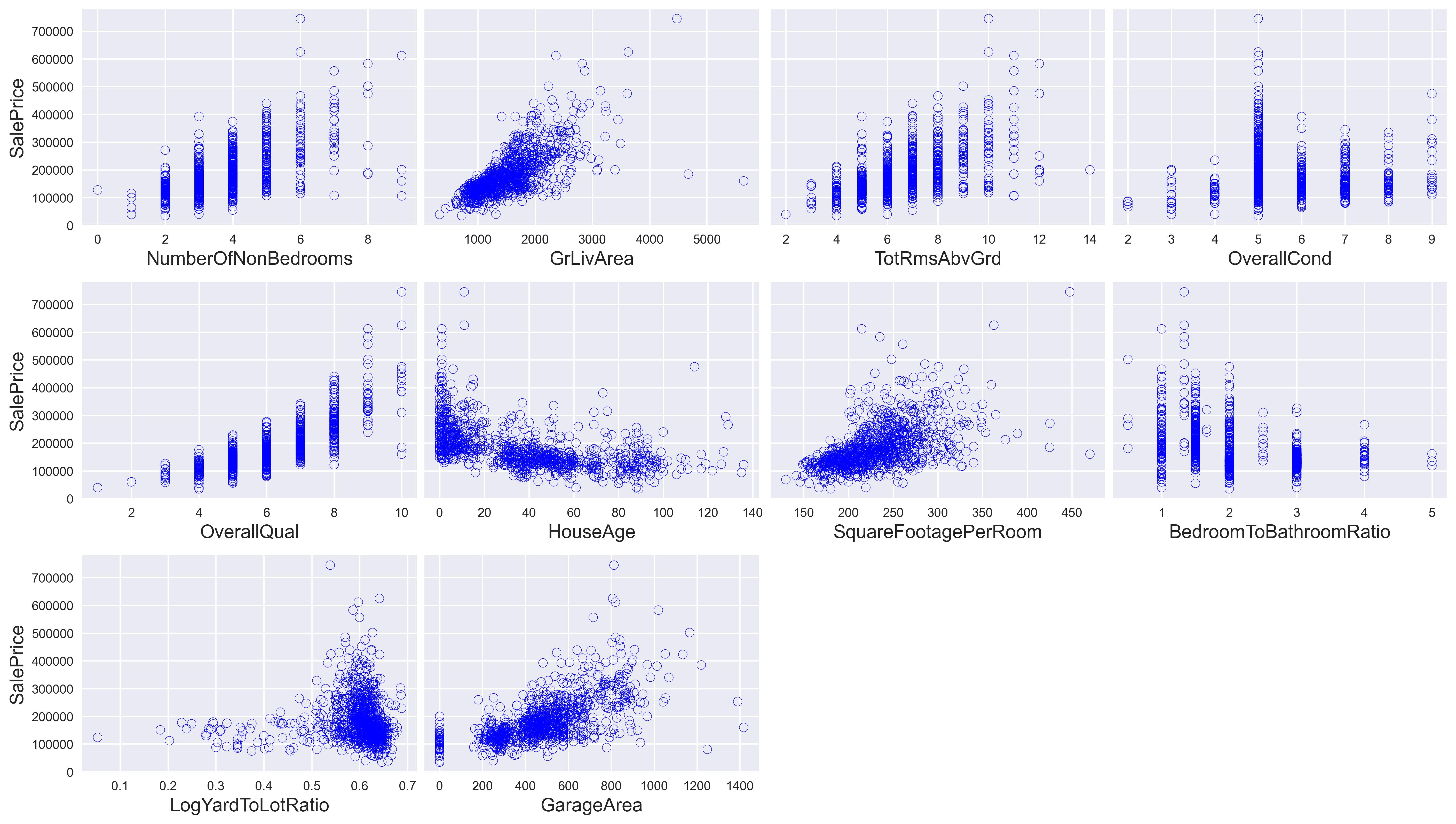
We can already see a few relationships here. For instance, OverallQual seems to have a positive, exponential impact on the housing price while HouseAge seems to have an exponentially decaying relationship to the housing price.
Now let’s get everything we need to start our backfitting algorithm. First and foremost (and because I know this only after playing with the code), we need to standardize our data by subtracting the mean of each feature and dividing by its standard deviation. The short answer to why we are doing this is that the backfitting algorithm does not converge with the current data as is.
# We need to keep a copy of the original dataframe for later
copy_of_original = copy.deepcopy(df)

mean = df[features + ["SalePrice"]].mean()
stdev = df[features + ["SalePrice"]].std()
df = (df[features + ["SalePrice"]] - mean) / stdev
Next, we need a few functions to construct our knots, truncated power basis, and second derivative basis. To simplify the calculations, we will use only 20 knots plus one additional knot for every 50 unique values if there are more than 20 unique values in the feature.
def spline_knots(values):
    unique_x = np.unique(values)

    if len(unique_x) <= 20:
        return unique_x

    return np.linspace(min(unique_x), max(unique_x), 20 + (len(unique_x) - 20) // 50)

def truncated_power_basis(values, knots):
    shape = (len(values), len(knots) + 4)
    X = np.ones(shape)

    for i, val in enumerate(values):
        X[i][1] = val
        X[i][2] = val**2
        X[i][3] = val**3

        for j, k in enumerate(knots, start=4):
            X[i][j] = max(0, val - k) ** 3

    return X

def f_double_prime_basis(values, knots):
    lb, ub = min(values), max(values)
    sample_points = np.linspace(lb, ub, 50)

    shape = (len(sample_points), len(knots) + 4)
    X_double_prime = np.zeros(shape)

    for i, val in enumerate(sample_points):
        X_double_prime[i][2] = 2
        X_double_prime[i][3] = 6 * val

        for j, k in enumerate(knots, start=4):
            X_double_prime[i][j] = 6 * max(0, val - k)

    return (X_double_prime, sample_points)
For estimation, our knots, basis functions, and second derivatives of the basis functions will not change, so all we have to do is create them once using the above functions. Let’s also create two lists called beta_old and beta_new to hold our spline coefficients’ current and previous estimates.
knots = [spline_knots(df[feat]) for feat in features]
basis = [truncated_power_basis(df[feat], knot) for feat, knot in zip(features, knots)]
derivative_basis = [
    f_double_prime_basis(df[feat], knot) for feat, knot in zip(features, knots)
]
beta_new = [np.zeros(len(knot) + 4) for knot in knots]
beta_old = [np.zeros(len(knot) + 4) for knot in knots]
We will use SciPy to minimize the PRSS above, subject to our constraints. To do that, we need a function that can be evaluated by the optimization method.
def function(x, target, base, integrand, lam):
    squared_residuals = np.square(target - base.dot(x))
    sum_of_squared_residuals = np.sum(squared_residuals)

    f_double_prime_x_squared, x_points= np.square(integrand[0].dot(x)), integrand[1]
    integral = scipy.integrate.simpson(f_double_prime_x_squared, x_points)

    return sum_of_squared_residuals + lam * integral
Now we are ready to get to the core of the algorithm. I will rewrite it below so that it’s easy to compare to the code. Remember that we have already done step 2 by setting the beta_new to zero for every function. We will use a value of $\lambda = 0.75$ to minimize the PRSS.
- Let $\hat{\alpha} = \frac{1}{N}\sum^{N}_{i=1}y_i$
- Set $\hat{f}_j = 0 \space\space \forall j$
-
For $j = 1, 2, \dots, p$:
\[\hat{f}_j \leftarrow S_j\bigg[\{y_i - \hat{\alpha} - \sum_{k\neq j} \hat{f}_k(x_{ik})\}_1^N\bigg]\] \[\hat{f}_j \leftarrow \hat{f}_j - \frac{1}{N}\sum^{N}_{i=1}\hat{f}_j(x_{ij})\] - Repeat step 3 until all functions have converged to within some tolerance.
# Set the vale of lambda and the convergence tolerance
lam = 0.75
tol = 1e-4
max_iter = 100

# We normalized all of our data, so alpha should be zero here anyways
alpha = df["SalePrice"].mean()
y_minus_alpha = (df["SalePrice"] - alpha).values
current_iter = 0
while current_iter < max_iter:

    for j, feature1 in enumerate(features):

        sum_of_other_f_k = np.zeros(len(df))
        for k, feature2 in enumerate(features):
            if j != k:
                sum_of_other_f_k += basis[k].dot(beta_new[k])

        # Set the constraints of the natural spline for the problem and the bounds
        # on b_2 and b_3.
        constr = (
            {"type": "eq", "fun": lambda x: np.sum(x[4:])},
            {"type": "eq", "fun": lambda x: x[4:].dot(knots[j])},
        )
        bnds = [
            (None, None) if (i != 2 and i != 3) else (0, 0)
            for i in range(len(beta_new[j]))
        ]

        target = y_minus_alpha - sum_of_other_f_k

        # Start the optimization problem.  When it finishes,
        # the result is stored in an attribute called x.  This
        # is the vector of betas.
        problem = scipy.optimize.minimize(
            function,
            beta_new[j],
            constraints=constr,
            bounds=bnds,
            args=(target, basis[j], derivative_basis[j], lam),
        )

        # subtract mean of the f_j from b_0
        problem.x[0] -= np.mean(basis[j].dot(problem.x))

        # Update betas
        beta_old[j] = beta_new[j]
        beta_new[j] = problem.x

    # Check for convergence
    converged = [np.linalg.norm(x_1 - x_0) for x_0, x_1 in zip(beta_old, beta_new)]
    if max(converged) <= tol:
        print("\nBackifitting algorithm has converged!\n")
        break

    current_iter += 1
    if current_iter == max_iter:
        print(
            "\nBackfitting algorithm failed to converge in {} iterations! Exiting!\n".format(
                max_iter
            )
        )
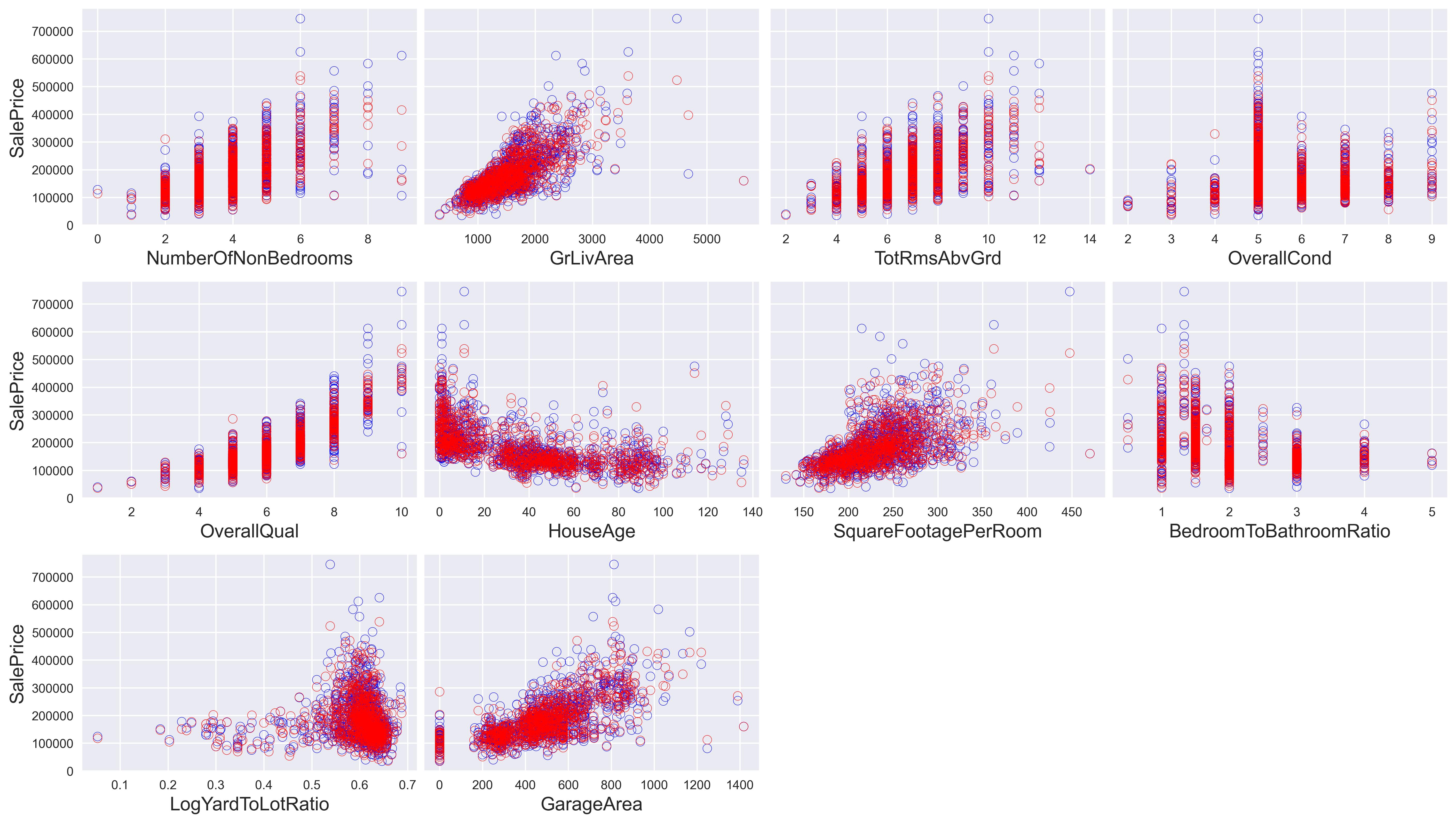
The above code will take a few minutes to run, but it will terminate successfully. Now we can plot the output of our predictions. The blue dots show the actual values of the housing prices, while the red dots show our predictions. It’s essential to keep in mind that because we scaled the data before the model estimation, we need to scale it back to its original form.
# Calculate the predictions for our training set.  We need to
# scale the data back to the original form by multiplying by
# the standard deviation and adding the mean to the entire array once.
prediction = np.zeros(len(df)) + mean["SalePrice"] + alpha
for feat, beta, base in zip(features, beta_new, basis):
    prediction += stdev["SalePrice"] * base.dot(beta)

fig, axes = plt.subplots(num_rows, num_columns, sharey=True)

fig.set_size_inches(16, 9)
fig.set_dpi(100)
fig.set_constrained_layout(True)
fig.set_constrained_layout_pads(hspace=0.05)

for index in range(num_rows * num_columns):
    row = index // num_columns
    col = index % num_columns

    if (row * num_columns + col) < len(features):
        x = copy_of_original[features[index]]
        y = copy_of_original["SalePrice"]

        axes[row, col].scatter(x, y, facecolors="none", edgecolors="b")
        axes[row, col].scatter(x, prediction, facecolors="none", edgecolors="r")
        axes[row, col].set(xlabel=features[index])
        if col == 0:
            axes[row, col].set(ylabel="SalePrice")

        axes[row, col].xaxis.label.set_size(10)
        axes[row, col].yaxis.label.set_size(10)
    else:
        axes[row, col].set_axis_off()
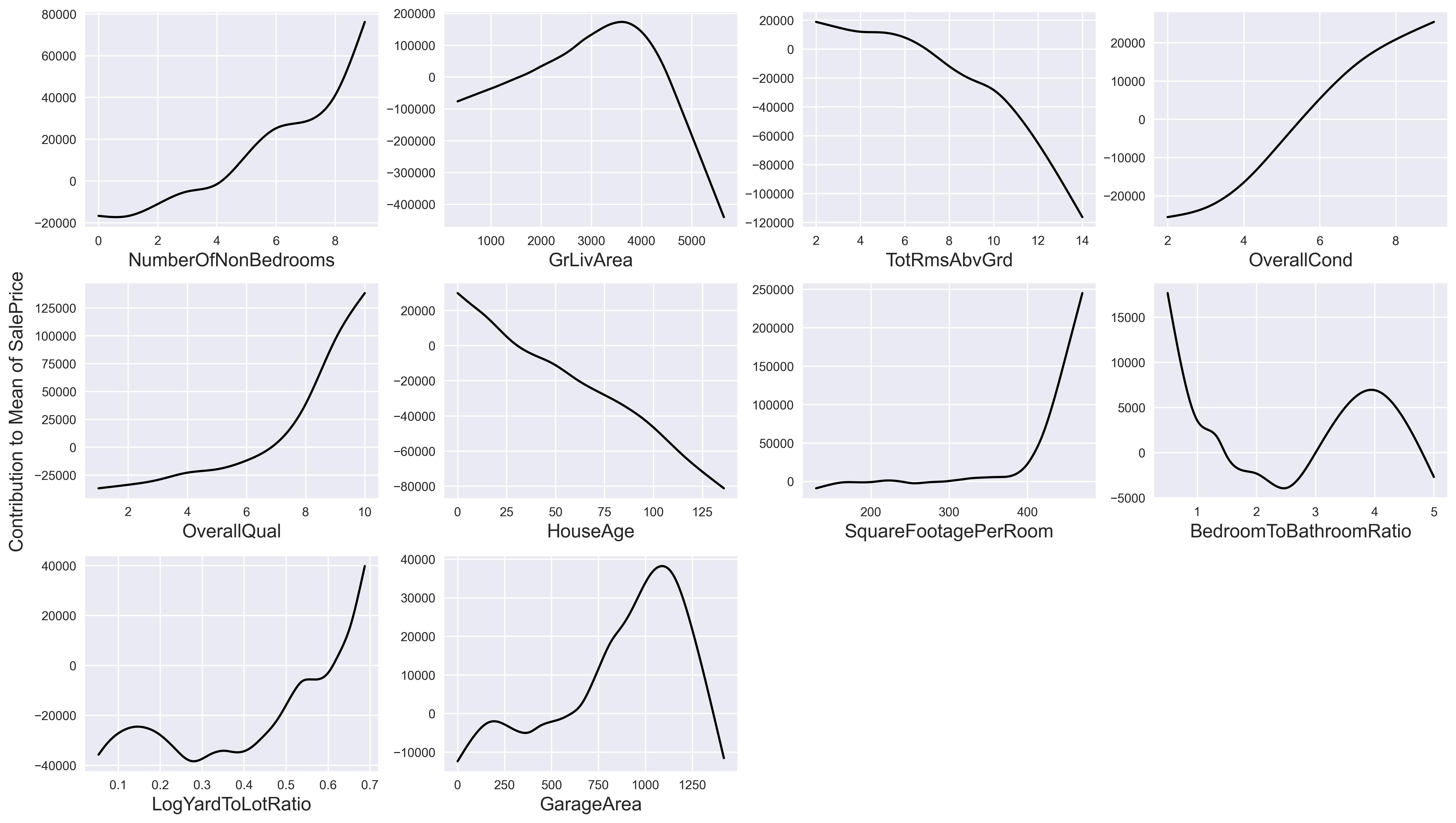
We can also view the contributions of each feature. Because we standardized the data before estimation, there is really no way to determine how much of the mean["SalePrice"] each feature contributes to the final price. However, we can visualize the contribution to or away from mean["SalePrice"].
fig, axes = plt.subplots(num_rows, num_columns, sharey=False)

fig.set_size_inches(16, 9)
fig.set_dpi(100)
fig.set_constrained_layout(True)
fig.set_constrained_layout_pads(hspace=0.05)
fig.supylabel('Contribution to Mean of SalePrice', size=15)

for index in range(num_rows * num_columns):
    row = index // num_columns
    col = index % num_columns

    if (row * num_columns + col) < len(features):
        x = np.linspace(min(df[features[index]]), max(df[features[index]]), 200)
        base = truncated_power_basis(x, knots[index])
        y = base.dot(beta_new[index]) * stdev["SalePrice"] + alpha

        axes[row, col].plot(
            x * stdev[features[index]] + mean[features[index]], y, c="black"
        )
        axes[row, col].set(xlabel=features[index])
        axes[row, col].xaxis.label.set_size(15)

    else:
        axes[row, col].set_axis_off()
Why We Had to Scale Our Data
While writing the code for this article, I realized that the backifitting algorithm was not converging, which was a big problem. Readers who have taken a numerical analysis course may draw some parallels between the backfitting algorithm and the Gauss-Seidel method for solving a system of equations. It turns out (and this is even an exercise in The Elements of Statistical Learning) that the backfitting algorithm can be formatted as the Gauss-Seidel method.
To quickly illustrate the method and its conditions for convergence, let us take an $n \times n$ matrix A. We want to solve the equation $Ax = b$ iteratively. The Gauss-Seidel algorithm poceeds by splitting $A$ into the following three $n \times n$ matrices.
\[\begin{align*} A = & \begin{bmatrix} a_{1,1} & a_{1,2} & \dots & a_{1, n-1} & a_{1, n} \\ a_{2, 1} & a_{2, 2} & \dots & a_{2, n-1} & a_{2, n}\\ \vdots & & \ddots & & \\ a_{n-1, 1} & a_{n-1, 2} & \dots & a_{n-1, n-1} & a_{n-1, n}\\ a_{n, 1} & a_{n, 2} & \dots & a_{n, n-1} & a_{n, n} \end{bmatrix}=\begin{bmatrix} a_{1,1} & 0 & \dots & 0 & 0 \\ 0 & a_{2, 2} & \dots & 0 & 0\\ \vdots & & \ddots & & \\ 0 & 0 & \dots & a_{n-1, n-1} & 0\\ 0 & 0 & \dots & 0 & a_{n, n} \end{bmatrix}\\ &\\ -&\begin{bmatrix} 0 & -a_{1,2} & \dots & -a_{1, n-1} & -a_{1, n} \\ 0 & 0 & \dots & -a_{2, n-1} & -a_{2, n}\\ \vdots & & \ddots & & \\ 0 & 0 & \dots & 0 & -a_{n-1, n}\\ 0 & 0 & \dots & 0 & 0 \end{bmatrix}-\begin{bmatrix} 0 & 0 & \dots & 0 & 0 \\ -a_{2, 1} & 0 & \dots & & 0\\ \vdots & & \ddots & & \\ -a_{n-1, 1} & -a_{n-1, 2} & \dots & 0 & 0\\ -a_{n, 1} & -a_{n, 2} & \dots & -a_{n, n-1} & 0 \end{bmatrix} \end{align*}\]So we can represent $A$ as the sum of the diagonal matrix $D$, the lower triangular matrix $L$, and the upper triangular matrix $U$. Distributing $x$ over $A$ yields
\[\begin{align*}Dx - (L + U)x = b\\Dx = (L + U) + b\\x = D^{-1}(L + U)x + D^{-1}b\end{align*}\]We make one replacement to arrive at the final method.
\[x_{k+1} = D^{-1}(L + U)x_k + D^{-1}b\]It turns out that this iterative method is only guaranteed to converge if the spectral radius, the maximum magnitude of the eigenvalues, of $D^{-1}(L + U)$ is less than 1.
If we use the natural cubic spline basis proposed in The Elements of Statistical Learning, it’s much easier to show the connection between the backfitting algorithm and the Gauss-Seidel method. Because I used numerical optimization in this article instead of finding the parameters based on a closed-form solution, I won’t go into the details of showing this.
Conclusion
In this article, we saw how to use natural cubic smoothing splines to minimize a penalized residual sum of squares function via nonlinear programming. Although The Elements of Statistical Learning provides a formula for construction spline terms that satisfy natural cubic spline conditions, we used numerical methods from SciPy to compute the parameters in the spline.
The good news is that we do not have to implement this algorithm from scratch whenever we want to build a generalized additive model. The Python package PyGam, written by Daniel Servén, offers a lot of flexibility and functionality for computing GAMs quickly and efficiently. The package can accommodate different types of link functions and makes determining feature contribution incredibly easy for both continuous and discrete features!
References
- Hastie, T., Friedman, J., & Tisbshirani, R. (2017). The elements of Statistical Learning: Data Mining, Inference, and prediction. Springer.
- Burden, Richard L., et al. “Chapter 7.” Numerical Analysis, 10th ed., Cengage Learning, Australia, 2016, pp. 456–463.
- Servén D., Brummitt C. (2018). pyGAM: Generalized Additive Models in Python. Zenodo. DOI: 10.5281/zenodo.1208723