Implementing a Simple Neural Network from Scratch
Artificial intelligence pervades our daily lives, from ChatGPT to mobile phone handwriting recognition. Even without delving into the mathematical intricacies, frameworks like PyTorch and TensorFlow simplify neural network implementation. Yet, understanding the mechanics behind these networks enhances our grasp of such frameworks. In this post, we’ll construct a basic feed-forward neural network to classify handwritten digits from the MNIST dataset, a repository of images spanning numbers 0 to 9. Note: familiarity with calculus and matrix multiplication is assumed. Let’s dive in.
The Structure of a Feed-Forward Neural Network
A typical neural network consists of two main components: nodes and weights. Nodes are often depicted as a stack of circles within a layer, each circle storing values in the network. Weights are illustrated as lines connecting nodes from one layer to the next, playing a crucial role in propagating data through the network. They determine the influence each node’s output has on the following layer. To visualize this concept, consider a simple graphical representation of a neural network.
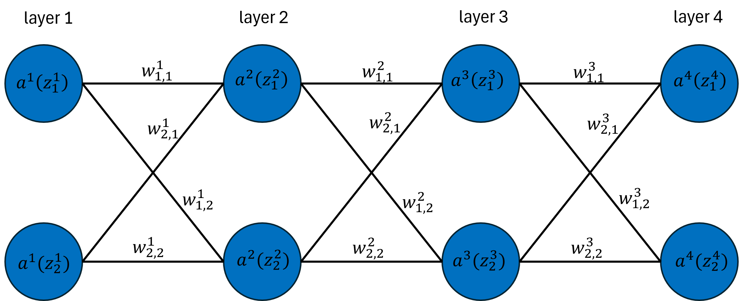
For the mathematical derivations of this article, we will work with the above network to get a sense of how neural networks function. To do that, we require some notation.
- $w^l_{i, j}$ is the weight from node $i$ in layer $l$ to node $j$ in layer $l + 1$.
- $\sigma^l$ is the activation function applied to $z^l_i$ before propagating the value to the next layer.
- $a^l_i$ is the activated value of node $i$ in layer $l$, i.e. $a^l_i = \sigma^l(z_i^l)$.
- $z^l_i$ is the pre-activated value of the node in layer $l$, which stores the linear combination of the weights and output from the previous node, i.e. \(z^2_1 = w^1_{1, 1}a^1_1 + w^1_{2,1}a^1_2\).
This diagram already seems involved, and some might notice that including an activation function only makes everything more computationally complicated, but the reason for including it will become clearer with an example of forward propagation.
Forward propagation is the process of feeding the neural network an input, passing this input through every layer, and obtaining an output. To illustrate this, let’s assume we have an input vector $\vec{x}=[x_1, x_2]$ that we want to feed into the network. A typical forward propagation cycle would be as follows.
- Set $z^1_1 = x_1$ and $z^1_2 = x_2$
- Compute $a^1_1 = \sigma^1(z^1_1)$ and $a^1_2 = \sigma^1(z^1_2)$
- Compute \(z^2_1 = w^1_{1, 1}a^1_1 + w^1_{2, 1}a^1_2\) and \(z^2_{2} = w^1_{1, 2}a^1_1 + w^1_{2,2}a^1_2\)
- Compute $a^2_1 = \sigma^2(z^2_1)$ and $a^2_2 = \sigma^2(z^2_2)$
Repeat steps 2 and 3 for the next layers until we reach the output layer. This process can be generalized to fit neural networks of arbitrary size.
We can make this a bit simpler by using vector and matrix notation as follows. Let $\vec{z}^l$ be the pre-activated values of the nodes in layer $l$ and $\mathbf{W}^l$ be the matrix of weights defined by
\[\mathbf{W}^l = \begin{bmatrix} w^l_{1, 1} & w^l_{2, 1} \\ w^l_{1, 2} & w^l_{2,2} \end{bmatrix}\]Then we can write the following
\[\vec{z}^2 = \begin{bmatrix} z^2 \\ z^2_1\end{bmatrix} = \begin{bmatrix} w^1_{1, 1}a^1_1 + w^1_{2,1}a^1_2\\ w^1_{1, 2}a^1_1 + w^1_{2,2}a^1_2\end{bmatrix}= \mathbf{W}^1\sigma^1(\vec{z}^1)\]where we apply the activation function $\sigma^1$ to each component of $\vec{z}^1$. In general, we have
\[\vec{z}^l = \mathbf{W}^{l-1}\sigma^{l - 1}(\vec{z}^{l - 1})\]The role of activation functions in a neural network becomes apparent when considering the consequences of their absence. If we were to eliminate the activation functions temporarily, the expression for the output layer could be written as
\[\vec{z}^L = \mathbf{W}^{L-1}\mathbf{W}^{L-2}\mathbf{W}^{L-3}\dots\mathbf{W}^{L-k}\vec{x}\]In this scenario, we observe a series of linear transformations applied to our input vector. Unfortunately, successive linear transformations only result in linear transformations, which can be limiting when the goal is to model nonlinear relationships. Including an activation function is essential to introducing nonlinearity, allowing the neural network to make more sophisticated predictions.
While forward propagation enables the computation of outputs given inputs in the network, it does not enhance the network’s performance. When initializing neural networks, the weights are typically set to small random values. Consequently, the output from propagating inputs through the network is random. To imbue the network with meaningful functionality, we need to train the network through backpropagation.
Deriving the Backpropagation Equations
Backpropagation is the process of iteratively updating the values of the weights to improve the performance of the neural network. To perform backpropagation we need two things: a loss function and an optimization algorithm. The loss function informs us about how “well” the network is doing. For example, in classic regression problems, a popular loss function is the mean squared error loss given by
\[L = \frac{1}{n}\sum_i(y_i - \hat{y}_i)^2\]where $\hat{y_i}$ is the predicted value for the $i^{th}$ observation and $y_i$ is the true value of the $i^{th}$ observation. There are many different kinds of loss functions, each suited to a specific type of problem. For now, we assume a general loss function, $L$, yet to be determined.
The optimization algorithm is the other key part of backpropagation. The goal is to update each weight by moving it a little bit in the direction that will reduce the total loss of the network. This can be mathematically formulated as
\[w^l_{i,j} \leftarrow w^l_{i,j} - \alpha \frac{\partial L}{\partial w^l_{i,j}}\]The term $\frac{\partial L}{\partial w^l_{i,j}}$ quantifies how $L$ changes with respect to the weight $w^l_{i,j}$. The parameter $\alpha$ is a positive real number determining the magnitude of the weight update. If$\frac{\partial L}{\partial w^l_{i,j}}$ is a large positive value, a reduction in the network’s total loss can be achieved by decreasing the weight by a fraction of this change. Conversely, if it’s a large negative value, increasing the weight can lead to loss reduction. In the scenario where $\frac{\partial L}{\partial w^l_{i,j}}$ equals zero, the weight remains unchanged. This situation signifies that the loss function, with respect to the specified weight, has reached a local minimum—a desirable outcome in the optimization process.
It would be convenient if we could, instead of updating one weight at a time, update every weight in a layer in one go. Ideally, we seek a matrix of derivatives $\mathbf{\partial W}^l$ given by
\[\mathbf{\partial W}^l = \begin{bmatrix} \frac{\partial L}{\partial w^l_{1, 1}} & \frac{\partial L}{\partial w^l_{2, 1}} & \dots & \frac{\partial L}{\partial w^l_{i, 1}} \\ \frac{\partial L}{\partial w^l_{1, 2}} & \frac{\partial L}{\partial w^l_{2, 2}} & \dots & \frac{\partial L}{\partial w^l_{i, 2}} \\ \vdots & \vdots & \ddots & \vdots \\ \frac{\partial L}{\partial w^l_{1, n}} & \frac{\partial L}{\partial w^l_{2, n}} & \dots & \frac{\partial L}{\partial w^l_{i, n}} \end{bmatrix}\]such that we can update the weight matrix $\mathbf{W}^l$ via
\[\mathbf{W}^l \leftarrow \mathbf{W}^l - \alpha \mathbf{\partial W}^l\]For our example network, updating the weights in the last layer would amount to the operation
\[\begin{bmatrix}w^3_{1, 1} & w^3_{2, 1} \\w^3_{1, 2} & w^3_{2, 2}\end{bmatrix} \leftarrow \begin{bmatrix}w^3_{1, 1} & w^3_{2, 1} \\w^3_{1, 2} & w^3_{2, 2}\end{bmatrix} - \alpha \begin{bmatrix} \frac{\partial L}{\partial w^3_{1, 1}} & \frac{\partial L}{\partial w^3_{2, 1}} \\ \frac{\partial L}{\partial w^3_{1, 2}} & \frac{\partial L}{\partial w^3_{2, 2}} \end{bmatrix}\]Let’s now determine how to calculate these partial derivatives for our example network. To do this, we need to make extensive use of the chain rule. For example, to calculate the partial derivative of $L$ with respect to $w^3_{1,1}$, we have
\[\frac{\partial L}{\partial w^3_{1,1}} = \frac{\partial L}{\partial a^4_1}\frac{\partial a^4_1}{\partial z^4_1}\frac{\partial z^4_1}{\partial w^3_{1,1}} + \frac{\partial L}{\partial a^4_2}\frac{\partial a^4_2}{\partial z^4_2}\frac{\partial z^4_2}{\partial w^3_{1,1}} = \frac{\partial L}{\partial a^4_1}\frac{\partial a^4_1}{\partial z^4_1}\frac{\partial z^4_1}{\partial w^3_{1,1}}\]where the last equality follows because \(\partial z^4_2/\partial w^3_{1,1} =0\) since \(w^3_{1,1}\) does not connect to the second node in the output layer. This result was obtained by starting at the output node and tracing a path back to our weight, taking partial derivatives using the chain rule along the way. So for our output layer we have the following matrix of partial derivatives
\[\mathbf{\partial W}^3 = \begin{bmatrix} \frac{\partial L}{\partial a^4_1}\frac{\partial a^4_1}{\partial z^4_1}\frac{\partial z^4_1}{\partial w^3_{1,1}} & \frac{\partial L}{\partial a^4_1}\frac{\partial a^4_1}{\partial z^4_1}\frac{\partial z^4_1}{\partial w^3_{2,1}}\\ \frac{\partial L}{\partial a^4_2}\frac{\partial a^4_2}{\partial z^4_2}\frac{\partial z^4_2}{\partial w^3_{1,2}} & \frac{\partial L}{\partial a^4_2}\frac{\partial a^4_2}{\partial z^4_2}\frac{\partial z^4_2}{\partial w^3_{2,2}} \end{bmatrix}\]We can further simplify this by using the fact that
\[\begin{align*} \frac{\partial z^4_1}{\partial w^3_{1,1}} &= \frac{\partial z^4_2}{\partial w^3_{1,2}} &&= a^3_1\\ \frac{\partial z^4_1}{\partial w^3_{2,1}} &= \frac{\partial z^4_2}{\partial w^3_{2,2}} &&= a^3_2\\ \end{align*}\]and using $a’^4_i$ to represent $\partial a^4_i / \partial z^4_i$ to rewrite the above as
\[\mathbf{\partial W}^3 = \begin{bmatrix} \frac{\partial L}{\partial a^4_1}a'^4_1a^3_1 & \frac{\partial L}{\partial a^4_1}a'^4_1a^3_2\\ \frac{\partial L}{\partial a^4_2}a'^4_2a^3_1 & \frac{\partial L}{\partial a^4_2}a'^4_2a^3_2 \end{bmatrix} =\left( \begin{bmatrix} \frac{\partial L}{\partial a^4_1}\\ \frac{\partial L}{\partial a^4_2} \end{bmatrix}\odot\begin{bmatrix} a'^4_1 \\ a'^4_2\end{bmatrix}\right)\begin{bmatrix}a^3_1 & a^3_2 \end{bmatrix}\]where $\odot$ represents element-wise multiplication. And just like that we have the matrix of partial derivatives for the final layer of weights.
Things start to get a little more complicated once we go further back in the network. Let’s compute the matrix following the paths in the network to each weight in the second to last layer.
\[\small{\mathbf{\partial W}^2 = \begin{bmatrix} \frac{\partial L}{\partial a^4_1} \frac{\partial a^4_1}{\partial z^4_1} \frac{\partial z^4_1}{\partial a^3_1} \frac{\partial a^3_1}{\partial z^3_1} \frac{\partial z^3_1}{\partial w^2_{1,1}} + \frac{\partial L}{\partial a^4_2} \frac{\partial a^4_2}{\partial z^4_2} \frac{\partial z^4_2}{\partial a^3_1} \frac{\partial a^3_1}{\partial z^3_1} \frac{\partial z^3_1}{\partial w^2_{1,1}} & \frac{\partial L}{\partial a^4_1} \frac{\partial a^4_1}{\partial z^4_1} \frac{\partial z^4_1}{\partial a^3_1} \frac{\partial a^3_1}{\partial z^3_1} \frac{\partial z^3_1}{\partial w^2_{2,1}} + \frac{\partial L}{\partial a^4_2} \frac{\partial a^4_2}{\partial z^4_2} \frac{\partial z^4_2}{\partial a^3_1} \frac{\partial a^3_1}{\partial z^3_1} \frac{\partial z^3_1}{\partial w^2_{2,1}} \\ \frac{\partial L}{\partial a^4_1} \frac{\partial a^4_1}{\partial z^4_1} \frac{\partial z^4_1}{\partial a^3_2} \frac{\partial a^3_2}{\partial z^3_2} \frac{\partial z^3_2}{\partial w^2_{1,2}} + \frac{\partial L}{\partial a^4_2} \frac{\partial a^4_2}{\partial z^4_2} \frac{\partial z^4_2}{\partial a^3_2} \frac{\partial a^3_2}{\partial z^3_2} \frac{\partial z^3_2}{\partial w^2_{1,2}} & \frac{\partial L}{\partial a^4_1} \frac{\partial a^4_1}{\partial z^4_1} \frac{\partial z^4_1}{\partial a^3_2} \frac{\partial a^3_2}{\partial z^3_2} \frac{\partial z^3_2}{\partial w^2_{2,2}} + \frac{\partial L}{\partial a^4_2} \frac{\partial a^4_2}{\partial z^4_2} \frac{\partial z^4_2}{\partial a^3_2} \frac{\partial a^3_2}{\partial z^3_2} \frac{\partial z^3_2}{\partial w^2_{2,2}} \end{bmatrix}}\] \[=\small{\begin{bmatrix} \frac{\partial L}{\partial a^4_1} a'^4_1 w^3_{1,1} a'^3_1 a^2_1 + \frac{\partial L}{\partial a^4_2} a'^4_2 w^3_{1,2} a'^3_1 a^2_1 & \frac{\partial L}{\partial a^4_1} a'^4_1 w^3_{1,1} a'^3_1 a^2_2 + \frac{\partial L}{\partial a^4_2} a'^4_2 w^3_{1,2} a'^3_1 a^2_2 \\ \frac{\partial L}{\partial a^4_1} a'^4_1 w^3_{2,1} a'^3_2 a^2_1 + \frac{\partial L}{\partial a^4_2} a'^4_2 w^3_{2,2} a'^3_2 a^2_1 & \frac{\partial L}{\partial a^4_1} a'^4_1 w^3_{2,1} a'^3_2 a^2_2 + \frac{\partial L}{\partial a^4_2} a'^4_2 w^3_{2,2} a'^3_2 a^2_2 \end{bmatrix}}\]Notice that this time there are two terms in each element of the matrix. This is because each output node is now a function of every weight in layer 2. With a little bit of work, we see that this matrix is equal to the following.
\[\mathbf{\partial W}^2 = \left(\begin{bmatrix} w^3_{1,1} & w^3_{1, 2} \\ w^3_{2, 1} & w^3_{2,2} \end{bmatrix} \begin{bmatrix}\frac{\partial L}{\partial a^4_1} \\ \frac{\partial L}{\partial a^4_2} \end{bmatrix} \odot \begin{bmatrix} a'^4_1 \\ a'^4_2 \end{bmatrix} \odot \begin{bmatrix} a'^3_1 \\ a'^3_2 \end{bmatrix} \right) \begin{bmatrix} a^2_1 & a^2_2 \end{bmatrix}\]Deriving $\mathbf{\partial W}^1$ will take even more work. We can simplify this process by realizing we have already done most of the work. Indeed, starting from the terms below
\[\frac{\partial L}{\partial z^3_1} = \frac{\partial L}{\partial a^4_1} \frac{\partial a^4_1}{\partial z^4_1} \frac{\partial z^4_1}{\partial a^3_1} \frac{\partial a^3_1}{\partial z^3_1} + \frac{\partial L}{\partial a^4_2} \frac{\partial a^4_2}{\partial z^4_2} \frac{\partial z^4_2}{\partial a^3_1} \frac{\partial a^3_1}{\partial z^3_1}\] \[\frac{\partial L}{\partial z^3_2} = \frac{\partial L}{\partial a^4_1} \frac{\partial a^4_1}{\partial z^4_1} \frac{\partial z^4_1}{\partial a^3_2} \frac{\partial a^3_2}{\partial z^3_2} + \frac{\partial L}{\partial a^4_2} \frac{\partial a^4_2}{\partial z^4_2} \frac{\partial z^4_2}{\partial a^3_2} \frac{\partial a^3_2}{\partial z^3_2}\]we can derive $\mathbf{\partial W}^1$ by extending the partial derivatives that we have already calculated
\[\mathbf{\partial W}^1=\begin{bmatrix} \frac{\partial L}{\partial z^3_1} \frac{\partial z^3_1}{\partial a^2_1} \frac{\partial a^2_1}{\partial z^2_1} \frac{\partial z^2_1}{\partial w^1_{1,1}} + \frac{\partial L}{\partial z^3_2} \frac{\partial z^3_2}{\partial a^2_1} \frac{\partial a^2_1}{\partial z^2_1} \frac{\partial z^2_1}{\partial w^1_{1,1}} & \frac{\partial L}{\partial z^3_1} \frac{\partial z^3_1}{\partial a^2_1} \frac{\partial a^2_1}{\partial z^2_1} \frac{\partial z^2_1}{\partial w^1_{2,1}} + \frac{\partial L}{\partial z^3_2} \frac{\partial z^3_2}{\partial a^2_1} \frac{\partial a^2_1}{\partial z^2_1} \frac{\partial z^2_1}{\partial w^1_{2,1}} \\ \frac{\partial L}{\partial z^3_1} \frac{\partial z^3_1}{\partial a^2_2} \frac{\partial a^2_2}{\partial z^2_2} \frac{\partial z^2_2}{\partial w^1_{1,2}} + \frac{\partial L}{\partial z^3_2} \frac{\partial z^3_2}{\partial a^2_2} \frac{\partial a^2_2}{\partial z^2_2} \frac{\partial z^2_2}{\partial w^1_{1,2}} & \frac{\partial L}{\partial z^3_1} \frac{\partial z^3_1}{\partial a^2_2} \frac{\partial a^2_2}{\partial z^2_2} \frac{\partial z^2_2}{\partial w^1_{2,2}} + \frac{\partial L}{\partial z^3_2} \frac{\partial z^3_2}{\partial a^2_2} \frac{\partial a^2_2}{\partial z^2_2} \frac{\partial z^2_2}{\partial w^1_{2,2}} \end{bmatrix}\] \[=\begin{bmatrix} \frac{\partial L}{\partial z^3_1} w^2_{1,1} a'^2_1 a^1_1 + \frac{\partial L}{\partial z^3_2} w^2_{1,2} a'^2_1 a^1_1 & \frac{\partial L}{\partial z^3_1} w^2_{1,1} a'^2_1 a^1_2 + \frac{\partial L}{\partial z^3_2} w^2_{1,2} a'^2_1 a^1_2 \\ \frac{\partial L}{\partial z^3_1} w^2_{2,1} a'^2_2 a^1_1 + \frac{\partial L}{\partial z^3_2} w^2_{2,2} a'^2_2 a^1_1 & \frac{\partial L}{\partial z^3_1} w^2_{2,1} a'^2_2 a^1_2 + \frac{\partial L}{\partial z^3_2} w^2_{2,2} a'^2_2 a^1_2 \end{bmatrix}\]And we can rewrite this as
\[\mathbf{\partial W}^1 = \left(\begin{bmatrix} w^2_{1,1} & w^2_{1, 2} \\ w^3_{2, 1} & w^2_{2,2} \end{bmatrix} \begin{bmatrix}\frac{\partial L}{\partial z^3_1} \\ \frac{\partial L}{\partial z^3_2}\end{bmatrix} \odot \begin{bmatrix} a'^2_1 \\ a'^2_2 \end{bmatrix} \right) \begin{bmatrix} a^1_1 & a^1_2 \end{bmatrix}\] \[= \small{\left(\left(\begin{bmatrix} w^2_{1,1} & w^2_{1, 2} \\ w^2_{2, 1} & w^2_{2,2} \end{bmatrix} \left(\begin{bmatrix} w^3_{1,1} & w^3_{1, 2} \\ w^3_{2, 1} & w^3_{2,2} \end{bmatrix} \begin{bmatrix}\frac{\partial L}{\partial a^4_1} \\ \frac{\partial L}{\partial a^4_2} \end{bmatrix} \odot \begin{bmatrix} a'^4_1 \\ a'^4_2 \end{bmatrix}\right) \odot \begin{bmatrix} a'^3_1 \\ a'^3_2 \end{bmatrix}\right) \odot \begin{bmatrix} a'^2_1 \\ a'^2_2 \end{bmatrix}\right) \begin{bmatrix} a^1_1 & a^1_2 \end{bmatrix}}\]Now we can see a pattern since we already computed most of the terms in parenthesis. Let’s generalize the steps as follows.
Step 1: Let $L$ denote the last layer in the neural network. Compute
\[\delta^L = \begin{bmatrix} \frac{\partial L}{\partial a^L_1} \\ \frac{\partial L}{\partial a^L_2} \\ \vdots \\ \frac{\partial L}{\partial a^L_{i-1}} \\ \frac{\partial L}{\partial a^L_i} \end{bmatrix} \odot \begin{bmatrix} \frac{\partial a^L_1}{\partial z^L_1} \\ \frac{\partial a^L_2}{\partial z^L_2} \\ \vdots \\ \frac{\partial a^L_{i-1}}{\partial z^L_{i-1}} \\ \frac{\partial a^L_{i}}{\partial z^L_i} \end{bmatrix}\]Step 2: For $l = L-1, L-2,\dots, 1$ compute
\[\mathbf{W}^{l} \leftarrow \mathbf{W}^{l} - \alpha \cdot \delta^{l + 1}{\vec{a}^{l}}^T\] \[\delta^l = {\mathbf{W}^{l}}^T\delta^{l+1} \odot \vec{a}'^{l}\]And there we have it, the mathematical details of the algorithm that make neural networks so powerful. It’s worth going back through the derivation of these equations for our example network to understand how the generalized equations work.
Implementing a Neural Network with NumPy
We will be implementing a simple feed-forward neural network to classify the MNIST dataset, which is a collection of 28x28 pixels representing handwritten digits and their corresponding labels.
To implement this network, we must first define a loss function. For problems where there are more than 2 categories possible (in this case we have 10 possible digits), a popular loss function is the cross-entropy loss function given by
\[L = -\sum_{k} y_k\cdot \ln{\hat{y}_k}\]where $y_k$ is a 1 if the class is of type $k$ and 0 otherwise and $\hat{y}_k$ represents the predicted probability that an observation is of class $k$. For the purposes of backpropagation, we will also need the gradient of $L$ with respect to $\hat{y}_k$. We can incorporate this into a Python function.
def cross_entropy(x, y, grad=False):
    """
    Calculates the cross-entropy loss between predicted (x) and true labels (y).

    Args:
        x: Predicted probabilities.
        y: True labels (one-hot encoded).
        grad: Boolean flag indicating whether to return the gradient (True) or loss (False).

    Returns:
        Cross-entropy loss if grad is False, otherwise the gradient of the loss.
    """

    # Clip target labels to avoid issues with log(0)
    x = np.clip(x, 1e-10, 1. - 1e-10)

    # Calculate cross-entropy loss
    if grad:
        return x - y  # Gradient of cross-entropy loss

    return -np.sum(y * np.log(x), axis=0)
Our network will make use of two activation functions, ReLU and Softmax. The ReLU activation is given by
\[ReLU(x) = \max(0,x)\]The ReLU function keeps only positive values, so it is a piecewise linear function that allows us to introduce some nonlinearity while keeping calculations cheap. The implementation of the ReLU function is as follows.
def relu(x, grad=False):
    """
    Implements the ReLU (Rectified Linear Unit) activation function.

    Args:
        x: Input value(s).
        grad: Boolean flag indicating whether to return the gradient (True) or activation (False).

    Returns:
        ReLU activation of x if grad is False, otherwise the ReLU gradient.
    """

    # Apply ReLU function: max(0, x)
    return np.maximum(0, x) if not grad else np.where(x > 0, 1.0, 0.0)
The Softmax function is the activation function that we will use in the last layer of the network. Its role is to assign a probability to each of the ten outputs, representing the probability of a certain digit aligning with the expected value. The Softmax function is given by
\[\text{Softmax}(x_i) = \frac{e^{x_i}}{\sum_{j=1}^{N} e^{x_j}}\]We can implement the Softmax function and its gradient with the following Python code.
def softmax(x, grad=False):
    """
    Implements the softmax function for classification problems.

    Args:
        x: Input value(s).
        grad: Boolean flag indicating whether to return the gradient (True) or activation (False).

    Returns:
        Softmax activation of x if grad is False, otherwise the softmax gradient.
    """

    # Calculate the exponentials of the input values for numerical stability
    exp = np.exp(np.maximum(np.minimum(x, 5), -5))

    # Prevent division by zero by adding a small constant to the denominator
    denominator = np.sum(exp, axis=0) + 1e-3

    # Calculate the softmax probabilities
    s = exp / denominator

    # Return activation or gradient based on the grad flag
    return s if not grad else np.multiply(s, 1. - s)
You may notice that we are bounding $x$ between -5 and 5. This is to avoid raising $e$ to too large of a power, which could result in numerical instability.
Now that we have our loss and activation functions out of the way, let’s implement the rest of the network. To align with conventional libraries like PyTorch and Tensorflow, let’s create a Layer class that will hold the weight matrices, the weight gradients, and necessary intermediate values.
class Layer:
    """
    Represents a basic neural network layer.

    Attributes:
        input_dim: Dimensionality of the input data.
        output_dim: Dimensionality of the output data.
        activation: Activation function to be applied to the layer's output.
        w: Weight matrix of the layer, initialized with random values.
        grad_w: Gradient of the weight matrix, used for training.
        x: Input data to the layer (stored for backpropagation).
        z: Weighted sum of the input before activation (stored for backpropagation).
        a: Activated output of the layer.
    """

    def __init__(self, input_dim, output_dim, activation=relu):
        """
        Initializes a new Layer object.

        Args:
            input_dim: Dimensionality of the input data.
            output_dim: Dimensionality of the output data.
            activation: Activation function to be applied to the layer's output (default: relu)
        """

        self.input_dim = input_dim
        self.output_dim = output_dim
        self.activation = activation

        # Initialize weight matrix with Xavier initialization for better convergence
        self.w = np.random.normal(scale=1.0 / np.sqrt(input_dim), size=(output_dim, input_dim)).astype(np.float32)
        self.grad_w = np.zeros_like(self.w).astype(np.float32)
        self.x = None
        self.z = None
        self.a = None

    def __call__(self, x):
        """
        Performs the forward pass through the layer.

        Args:
            x: Input data to the layer.

        Returns:
            Activated output of the layer.
        """

        self.x = x  # Store the input for backpropagation
        self.z = np.dot(self.w, x)  # Calculate the weighted sum
        self.a = self.activation(self.z)  # Apply activation function
        return self.a
Now we create a NeuralNetwork class that will do forward and backward propagation as well as calculating the loss.
class NeuralNetwork:
    """
    Represents a basic neural network architecture.

    Attributes:
        learning_rate: Learning rate for gradient updates during training.
        batch_size: Size of the data batch used for training.
        layers: List of `Layer` objects representing the network's layers.
        predictions: Network's predicted outputs during the last forward pass (internal use).
        actuals: True labels during the last forward pass (internal use).
        current_loss: Loss value calculated during the last forward pass (internal use).
    """

    def __init__(self, learning_rate=0.01, batch_size=32, loss_function=cross_entropy):
        """
        Initializes a new NeuralNetwork object.

        Args:
            learning_rate: Learning rate for gradient updates during training (default: 0.01).
            batch_size: Size of the data batch used for training (default: 32).
            loss_function: The function used to calculate loss (default: cross_entropy).
        """
        self.learning_rate = learning_rate
        self.batch_size = batch_size
        self.loss_function = loss_function
        self.layers = []  # List to hold network layers

        # Internal variables to store network outputs for loss calculation
        self.predictions = None
        self.actuals = None
        self.current_loss = None

    def __call__(self, x):
        """
        Performs a forward pass through the network.

        Args:
            x: Input data to the network.

        Returns:
            Activated output of the last layer in the network.
        """
        for layer in self.layers:
            x = layer(x)  # Pass input through each layer
        return x

    def __add__(self, layer):
        """
        Efficiently adds a Layer object to the network.

        Args:
            layer: The Layer object to be added to the network.

        Raises:
            AssertionError: If the input and output dimensions of consecutive layers are incompatible.
        """
        if isinstance(layer, Layer):
            if not self.layers:
                self.layers.append(layer)
            else:
                # Ensure compatible dimensions between layers
                assert layer.w.shape[1] == self.layers[-1].w.shape[0], "Incompatible layer dimensions!"
                self.layers.append(layer)
        return self

    def loss(self, predictions, actuals):
        """
        Calculates and stores the loss between predicted and actual outputs.

        Args:
            predictions: Network's predicted outputs.
            actuals: True labels for the data.

        Returns:
            The calculated loss value.
        """
        self.predictions = predictions
        self.actuals = actuals
        self.current_loss = np.mean(self.loss_function(predictions, actuals))  # Average cross-entropy loss
        return self.current_loss

    def backwards(self):
        """
        Performs backpropagation to update weights of the network based on the calculated loss.
        """
        # Calculate the gradient of the loss with respect to the network's predictions
        loss_grad = cross_entropy(self.predictions, self.actuals, grad=True)
        # Calculate the gradient of the activation function of the last layer
        activation_grad = self.layers[-1].activation(self.layers[-1].z, grad=True)

        # Compute the delta, which is the product of the loss gradient and activation gradient
        delta = loss_grad * activation_grad
        # Reshape delta for compatibility with matrix multiplication
        delta = delta.T.reshape(self.batch_size, -1, 1)

        # Compute the gradient of the weights of the last layer
        prev_activation = self.layers[-1].x.T.reshape(self.batch_size, 1, -1)
        self.layers[-1].dw = np.mean(delta * prev_activation, axis=0)

        # Backpropagate through the layers, starting from the second-to-last layer
        for i in range(2, len(self.layers) + 1):
            # Transpose weights for matrix multiplication
            weights_transpose = self.layers[-i + 1].w.transpose()

            # Compute the gradient of the activation function of the current layer
            z = self.layers[-i].z
            activation_grad = self.layers[-i].activation(z, grad=True)
            activation_grad = activation_grad.T.reshape(self.batch_size, -1, 1)

            # Update delta using the chain rule
            delta = np.matmul(weights_transpose, delta) * activation_grad

            # Compute the gradient of the weights of the current layer
            prev_activation = self.layers[-i].x.T.reshape(self.batch_size, 1, -1)
            self.layers[-i].dw = np.mean(np.matmul(delta, prev_activation), axis=0)

        # Update weights of all layers using gradient descent
        for layer in self.layers:
            layer.w = layer.w - self.learning_rate * layer.dw
The backwards method implements backpropagation according to the equations we derived above. The main difference between the mathematics and the implementation is that I am taking advantage of mini-batch gradient descent, which samples a batch of data, calculates the gradient matrix for each sample in the batch, and then averages those gradient matrices for the weight update. These operations are done in the background by NumPy using the rules of broadcasting.
Let’s go ahead and use our model to classify some digits. We will read a file called mnist_train.csv, where the structure is such that each row corresponds to a digit with the first column being the label, and the next 784 columns being the flattened 28x28 image.
file = r"MNIST_CSV\mnist_train.csv"
data = pd.read_csv(file, header=None).values.astype(np.float32)
samples = [(data[i, 1:] / 255, np.eye(10)[int(data[i, 0])].astype(np.float32)) for i in range(len(data))]
We store each row’s data in a tuple and divide every pixel value by 255 to normalize the data between 0 and 1. This helps avoid overflow errors in the network. We have also converted the label into a one-hot encoded vector, i.e. a vector of length 10 with the index of the label set to 1 and zero otherwise. Next, we create a model and test it on our training data.
np.random.seed(10_000)
random.seed(10_000)
model = NeuralNetwork(learning_rate=.95, batch_size=64)
l1 = Layer(784, 50, relu)
l2 = Layer(50, 20, relu)
l3 = Layer(20, 10, softmax)
model += l1
model += l2
model += l3
epochs = 10_000
losses = []
for i in trange(epochs, ncols=1000):
batch = random.sample(samples, model.batch_size)
X = np.column_stack([b[0] for b in batch]).astype(np.float32)
Y = np.column_stack([b[1] for b in batch]).astype(np.float32)
pred = model(X)
loss = model.loss(pred, Y)
losses.append(loss)
model.backwards()
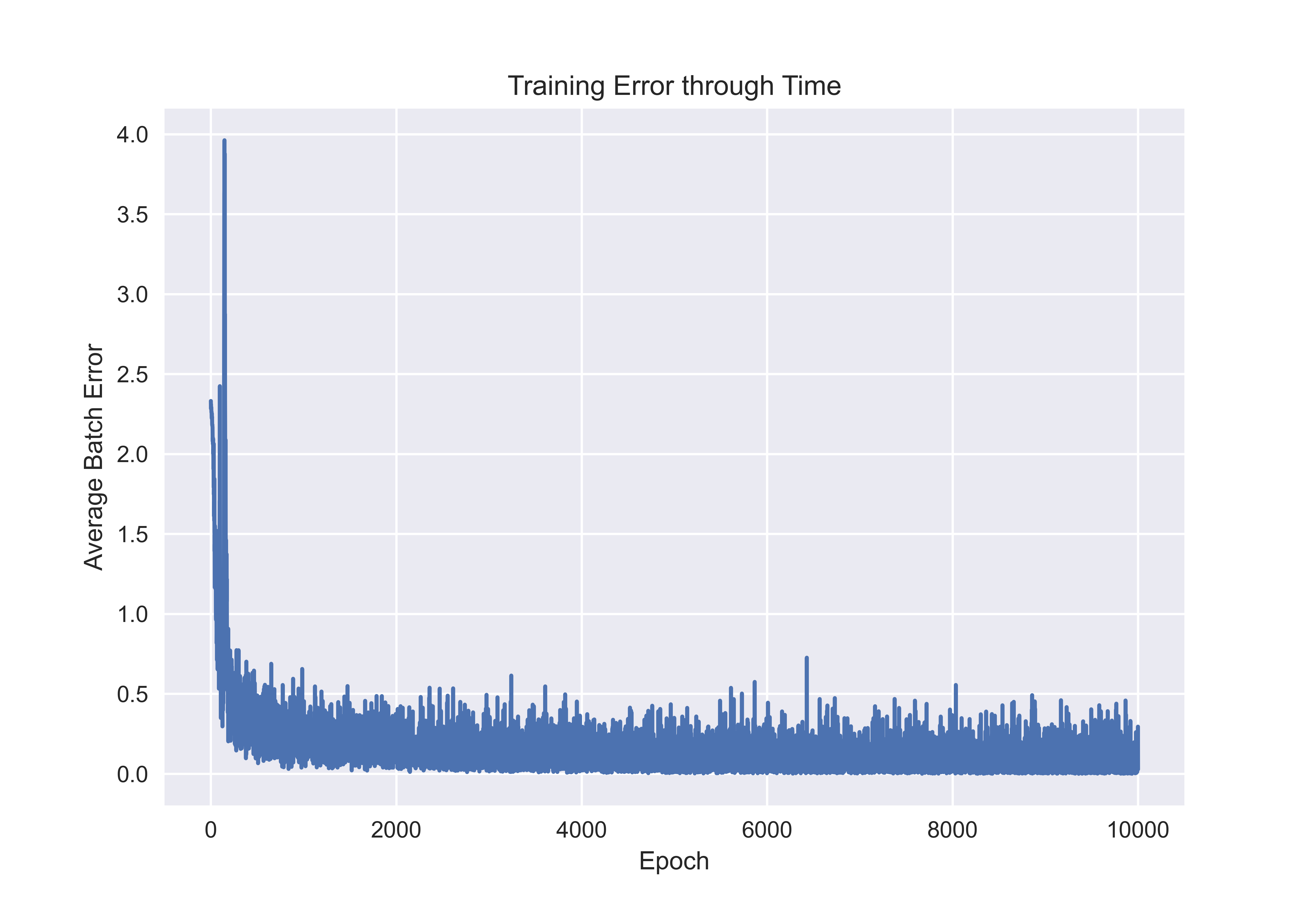
plt.plot(losses)
plt.xlabel("Epoch")
plt.ylabel("Average Batch Error")
plt.title("Training Error through Time")
plt.savefig('error.png', dpi=600)
When you run this code, you should get the following graph or something very similar. We see that the error drops off rapidly in training, which is a good indication that our network is learning well. However, it should be noted that convergence depends on several factors including the learning rate.
The full code for the neural network implementation can be found in this repository.
Conclusion
In this article, we derived the backpropagation equations for feed-forward neural networks and wrote a naive implementation to classify digits in the MNIST dataset. Nevertheless, some improvements can be made to the implementation
- Introduce bias terms: Introducing bias terms allows neural networks to better model complex relationships between inputs and outputs by shifting activation functions, enhancing the network’s ability to learn.
- Use learning rate scheduling: Utilizing learning rate scheduling optimizes training by dynamically adjusting the learning rate over epochs, allowing for faster convergence and better generalization.
- Consider different optimizers: Considering different optimizers such as Adam, RMSprop, or SGD with momentum can improve training efficiency and performance by adapting gradient descent algorithms to better suit the data and model architecture.
It is also worth mentioning that many machine-learning frameworks do not explicitly perform backpropagation through matrix multiplication. Instead, they use an algorithm known as autograd, that keeps a graph representation of the network and traverses that to compute the derivatives. More information about autograd is available here.